

Sea ice models compute the thickness of sea ice and the area covered with it based on physical equations, which describe the relevant natural processes. Some processes, however, cannot be fully resolved and involve the use of so-called parameterizations, which allow simulating effects of processes on scales smaller than the model grid. As an example sea ice ridges of up to 10 m thickness are observed to occur as part of otherwise considerably thinner ice floes. These thickness differences in nature can occur on a distance of several meters, whereas sea ice models use grid resolutions of several kilometres. As a consequence the sea ice thickness distribution, i.e. the abundance of different thickness categories within the area of a grid box, has to be parameterized.
Since the thickness of the sea ice determines how much heat exchange can take place between the atmosphere and the ocean, a realistic sea ice thickness distribution is essential. Many sea ice models parameterize the sub-grid thickness distribution with a probability density function (pdf) of different ice thickness categories (Fig. 1). The number of categories and the shape of the pdf have a strong influence on the simulated ice volume. Many models use a uniformly shaped pdf with seven categories as suggested by Hibler [1984]. We found that a distribution parameterization with 15 sea ice thickness categories, which are based on observations ([Castro-Morales et al., 2014]), leads to simulations with a more realistic sea ice area consistent to satellite derived observations (OSI SAF; Global sea ice concentration reprocessing dataset 1978-2009 (v1.1, 2011); Norwegian and Danish Meteorological Institutes. Available from http://osisaf.met.no.). Other parameterizations also have a significant effect. Even with a very simple ice thickness category distribution (every category is equally likely to occur) better results can be achieved when the model is tuned with additional sea ice parameters.
One such parameter is h0, which parameterizes how newly formed ice is horizontally distributed when ice formation sets in. Even when using a very simple ‘one ice thickness category’ parameterization a realistic sea ice volume can be achieved when making h0 not constant, which is usually the case, but let it vary over time and space as used in Notz et al. [2013].
These examples show, that the chosen combination of parameterizations in a model offer the potential for resulting in more realistic model results, but pose the difficulty of ambiguous results at the same time. These combinations are also a source of uncertainty in model simulations and improvement.
Kathrin Riemann-Campe1, Rüdiger Gerdes1, Cornelia Köberle1, Michael Karcher1,2, Frank Kauker1,2, 1Alfred-Wegener-Institut; 2O.A.Sys
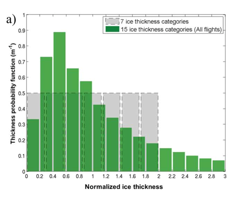
Figure1: Different ice thickness distributions: the grey distribution is based on Hibler [1984] and is used in many models; the green distribution is based on airborne EM-bird measurements. Figure modified from Castro-Morales et al. [2014]